HoloFoodR: a statistical programming framework for holo-omics data integration workflows
2026-02-10
Source:vignettes/articles/case_study.Rmd
case_study.RmdIntroduction
HoloFood database is a large collection of holo-omic and multi-omic data from two animal systems, chicken and salmon. It was created by the HoloFood consortium. One of its objectives is to study the interactions between animal systems, their microbiomes, and feed additives to optimize the diet strategies of these farm animals.
For make it easily accessible, the developers provide an Application Programming Interface (API) that permits interaction with programming languages, such as R or Python.
We improve the accessibility by creating the HoloFoodR package that simplifies API interaction and assists translating raw database data into R/Bioconductor data containers, connecting to a vast ecosystem of bioinformatics R packages.
We do not aim to demonstrate HoloFoodR in isolation from the rest of the ecosystem, but to showcase the possibility of data integration from other databases, such as MGnify, which holds metagenomic data. Furthermore, we provide a workflow from data exploration to advanced machine learning and multi-omics, offering a practical example for readers.
Our main study questions are:
- How does treatment influence the gut microbiota of salmon?
- Do gut flora and fatty acids composition evolve over time?
- Is there a relationship between gut microbiota and the fatty acid composition in muscle tissue?
# List of packages that we need
packages <- c(
    "dplyr", "DT", "ggsignif", "HoloFoodR", "MGnifyR", "mia", "miaViz", "MOFA2",
    "patchwork", "reticulate", "scater", "shadowtext"
)

# Load all packages into session. Stop if there are packages that were not
# successfully loaded
pkgs_not_loaded <- !sapply(packages, function(pkg){
    suppressPackageStartupMessages(require(pkg, character.only = TRUE))
})
pkgs_not_loaded <- names(pkgs_not_loaded)[pkgs_not_loaded]
if (length(pkgs_not_loaded) > 0) {
    stop("Error in loading the following packages into the session: '",
        paste0(pkgs_not_loaded, collapse = "', '"), "'")
}
Import data
We start the workflow from data retrieval. We will use salmon data and its associated fatty acid and metagenomic amplicon as an example.
Retrieve HoloFood data
First of all, we have to query the HoloFood database to retrieve the salmon accession numbers.
# Get salmon samples
salmons <- HoloFoodR::doQuery("animals", system = "salmon", use.cache = TRUE)

# Get only the data that has both metagenomic amplicon and fatty acid
# data
salmons <- salmons |>
    filter(fatty_acids == TRUE & metagenomic_amplicon == TRUE)

colnames(salmons)
Next, we can retrieve the data associated with each salmon.
# Get salmon data
salmon_data <- HoloFoodR::getData(
    accession.type = "animals",
    accession = salmons[["accession"]],
    use.cache = TRUE
)

# Get salmon samples
salmon_samples <- salmon_data[["samples"]]

# Get sample IDs
salmon_sample_ids <- unique(salmon_samples[["accession"]])

head(salmon_sample_ids)
The data returned above is a list of all sample accession numbers that are associated with all salmons. For example, metagenomic amplicon samples, such as SAMEA112750580 or fatty acid samples, SAMEA112950027.
We can use these accession numbers to fetch the data associated with
each sample type and store them as experiments in a
MultiAssayExperiment (MAE) object.
# Get salmon <- experiments as MAE object
mae <- HoloFoodR::getResult(
    salmon_sample_ids,
    use.cache = TRUE
)
Fetch metagenomic data from MGnify
HoloFood database does not include the data for metagenomic data. This data can be retrieved from the MGnify portal. For this purpose, we will use MGnifyR package, which in a similar fashion to HoloFoodR, allows simple interaction with MGnify API.
# Create MGnify object
mg <- MgnifyClient(
    useCache = TRUE,
    cacheDir = ".MGnifyR_cache"
)

# Select only metagenomic_amplicon sample type
metagenomic_salmon_samples <- salmon_samples |>
    filter(sample_type == "metagenomic_amplicon")

# Search for sample IDs in MGnify database
salmon_analysis_ids <- searchAnalysis(
    mg,
    type = "samples",
    metagenomic_salmon_samples[["accession"]]
)
salmon_analysis_ids character vector holds associations
of HoloFood metagenomic amplicon accession numbers (SAMEAxxxxxx) to
their counterparts in MGnify database (MGYAxxxxxx).
# Get metagenomic taxonomic data for salmon from MGnify
tse <- MGnifyR::getResult(
    mg,
    accession = salmon_analysis_ids,
    get.func = FALSE
)
Data fetched from MGnify has MGnify-specific identifiers. We have to
first rename samples with HoloFood specific ID and then add the data to
MultiAssayExperiment combining all the data.
# Add MGnify results to HoloFood data
mae <- addMGnify(tse, mae)
#> Warning: 'experiments' dropped; see 'drops()'
#> harmonizing input:
#>   removing 189 sampleMap rows not in names(experiments)
#> harmonizing input:
#>   removing 189 sampleMap rows not in names(experiments)
Now we have retrieved all the data that we are interested in this workflow.
Data preprocess
Data cleaning is one of the most time-consuming and most important steps in data analysis. For instance, we need to handle missing data, transform data assays, and agglomerate the data.
In the next steps, we will:
- Filter data
- Ensure that the data is in correct format for analysis
- Agglomerate data
- Transform data
Wrangle the data
Below we see upset plot that summarizes the available experiments and how samples overlap between them.
upset_plot <- upsetSamples(mae)
#> Warning: `aes_string()` was deprecated in ggplot2 3.0.0.
#> ℹ Please use tidy evaluation idioms with `aes()`.
#> ℹ See also `vignette("ggplot2-in-packages")` for more information.
#> ℹ The deprecated feature was likely used in the UpSetR package.
#>   Please report the issue to the authors.
#> This warning is displayed once per session.
#> Call `lifecycle::last_lifecycle_warnings()` to see where this warning was
#> generated.
#> Warning: Using `size` aesthetic for lines was deprecated in ggplot2 3.4.0.
#> ℹ Please use `linewidth` instead.
#> ℹ The deprecated feature was likely used in the UpSetR package.
#>   Please report the issue to the authors.
#> This warning is displayed once per session.
#> Call `lifecycle::last_lifecycle_warnings()` to see where this warning was
#> generated.
#> Warning: The `size` argument of `element_line()` is deprecated as of ggplot2 3.4.0.
#> ℹ Please use the `linewidth` argument instead.
#> ℹ The deprecated feature was likely used in the UpSetR package.
#>   Please report the issue to the authors.
#> This warning is displayed once per session.
#> Call `lifecycle::last_lifecycle_warnings()` to see where this warning was
#> generated.
upset_plot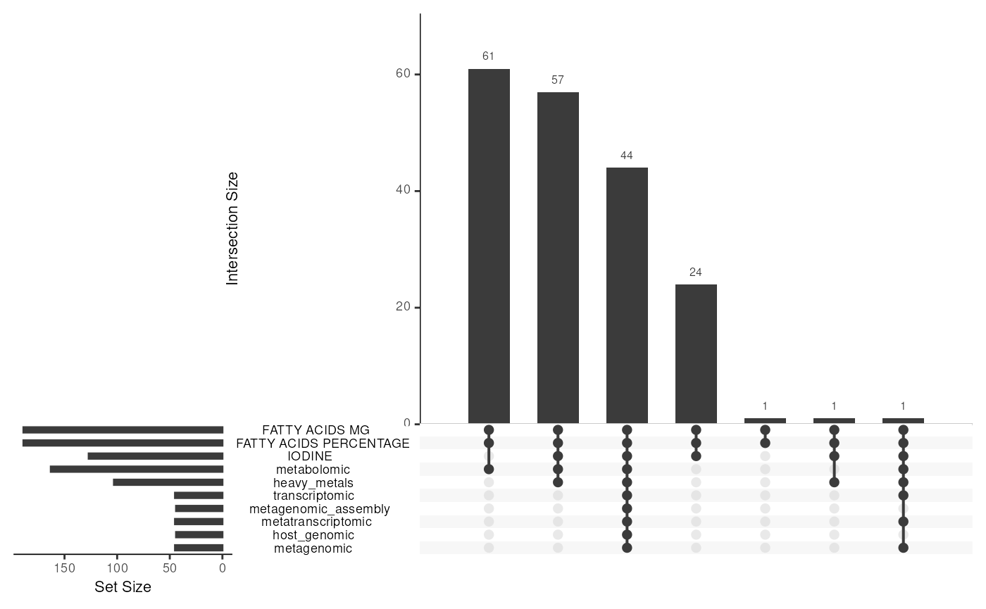
The distribution of experiments in the dataset, along with the number of samples in each experiment.
For demonstration purposes, we will focus on investigating fatty acids and metagenomic data within the trial A performed by the HoloFood consortium. This trial the health effects of fermented seaweed added to the diet of salmons. The following script subsets the data to include aforementioned data.
# Harmonize experiment names
names(mae) <- names(mae) |>
    tolower() |>
    gsub(pattern = " ", replacement = "_")

# Fetch only experiments that we need
mae <- mae[, , c("fatty_acids_mg", "metagenomic")]
#> Warning: 'experiments' dropped; see 'drops()'
#> harmonizing input:
#>   removing 934 sampleMap rows not in names(experiments)
names(mae) <- c("fatty_acids", "metagenomic")
# Filter MAE object to include only Trial A
mae <- mae[, colData(mae)[["Trial code"]] == "SA", ]
Some values of fatty acids are under detection thresholds. We assume them to be zeroes. Moreover, the data includes a feature that just states from where the fatty acids were collected. We remove this feature to ensure that the assay contains only numeric values.
# From metabolomic data, remove organ-fatty acids row because it only contains a
# string value "muscle" which denotes where the sample was drawn from
tse <- mae[[1]]
tse <- tse[!(rowData(tse)[["marker.name"]] %in% c("Organ-fatty acids")), ]
mae[[1]] <- tse

# Transform matrix to numeric. Some values are "< 0.01"
# If a number is < 0.01, assume it to be 0
assay <- assay(mae[[1]], "counts")
assay[assay == "<0.01"] <- 0
assay <- apply(assay, c(1, 2), function(x) as.numeric(gsub(",", ".", x)))

# Reassign assay back to MAE
assay(mae[[1]], "counts") <- assay
Moreover, we wrangle the sample metadata so that it includes all necessary information.
# Add time points
timepoints <- colData(mae[[2]])
timepoints <- timepoints[
    match(timepoints[["animal"]], rownames(colData(mae))), ]
timepoints <- ifelse(timepoints[["trial.timepoint"]] == 0, "start", "end")
timepoints <- factor(timepoints, levels = c("start", "end"))
colData(mae)[["timepoint"]] <- timepoints

# Add treatment groups
colData(mae)[["study_group"]] <- ifelse(
    colData(mae)[["Treatment concentration"]]>0, "treatment", "control")
colData(mae)[colData(mae)[["timepoint"]] == "start" , "study_group"] <-
    "control"

# Add animal metadata to separate experiments
mae[[1]] <- getWithColData(mae, 1)
#> Warning: Ignoring redundant column names in 'colData(x)': canonical_url,
#> marker.type
mae[[2]] <- getWithColData(mae, 2)
#> Warning: Ignoring redundant column names in 'colData(x)': canonical_url,
#> marker.type
Filtering and agglomeration
Next, we can agglomerate features by prevalence to reduce the number of low-abundant taxa and contaminants.
First, we visualize prevalence distribution of taxa with a histogram to decide the prevalence threshold to use. We use 0.2% detection level to filter out extremely low-abundant genera.
# Add relative abundance data
mae[[2]] <- transformAssay(mae[[2]], method = "relabundance")

# Compute prevalence of relative abundance of microbial genera at detection
# level of 0.1%
prevalence <- getPrevalence(
    mae[[2]],
    rank = "Genus",
    assay.type = "relabundance",
    na.rm = TRUE,
    sort = TRUE,
    detection = 0.2 / 100
)

# Exclude microbes with 0 prevalence
prevalence <- prevalence[prevalence != 0]

hist(prevalence, main = "", xlab = "Prevalence")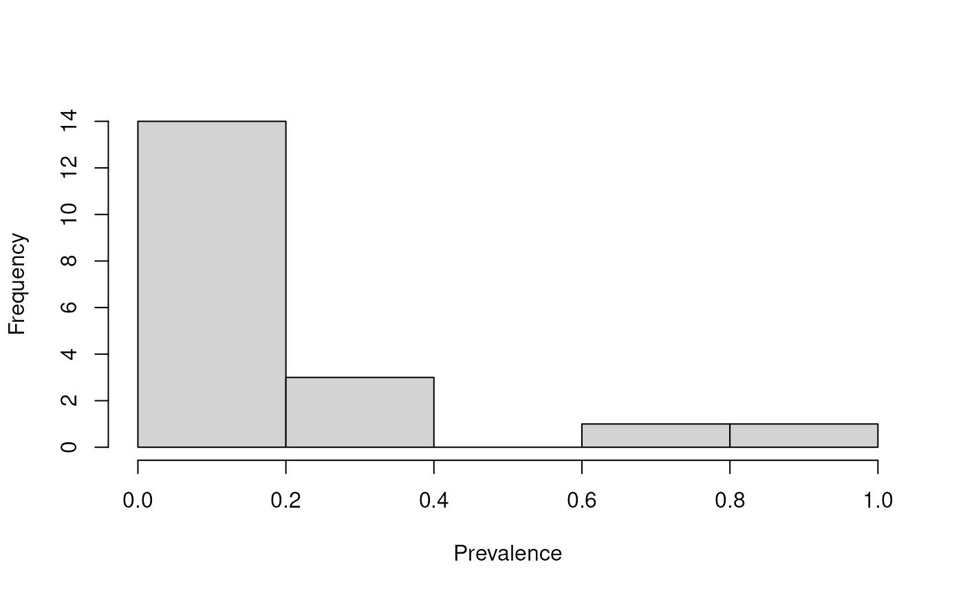
The prevalence of microbial genera across samples.
We can also look at the raw prevalence numbers.
# Sort prevalence in decreasing order
sort(prevalence, decreasing = TRUE) |> head(10)
#>     Mycoplasma Photobacterium     Aliivibrio  Cetobacterium         Vibrio
#>      0.9777778      0.7111111      0.4000000      0.2666667      0.2444444
#> Ammopiptanthus    Francisella    Paucibacter  Mycobacterium       Medicago
#>      0.1555556      0.1333333      0.1111111      0.1111111      0.1111111
Mycoplasma is present in all samples, which is not surprising as this genus was found to be one of the most common in salmon intestine (see Zarkasi et al. (2014)).
We then agglomerate our data by prevalence and by taxonomic rank to obtain group all genera which are below the specified thresholds to the “Other” group. This step is necessary to ensure that we only work with the most relevant taxa, while not excluding the rest of data points. We use thresholds 20% and 0.2% for prevalence and detection, respectively.
# Agglomerate by prevalence by genus
altExp(mae[[2]], "prev_genus") <- agglomerateByPrevalence(
    mae[[2]],
    assay.type = "relabundance",
    rank = "Genus",
    prevalence = 20 / 100,
    detection = 0.2 / 100
)
Due to the limited number of samples, we also filter the fatty acid data to include only those fatty acids that show variation within the dataset. The rationale is that if a fatty acid does not vary, it cannot exhibit differences between groups. We can find out a good threshold for the cutoff with a histogram of standard deviations of fatty acid abundances.
rowData(mae[[1]])[["sd"]] <- rowSds(assay(mae[[1]], "counts"), na.rm = TRUE)
hist(rowData(mae[[1]])[["sd"]], breaks = 30, main = "",
    xlab = "Standard deviation")

# Increase the number of x axis ticks
x_labels <- seq(from = min(assay(mae[[1]])), to = max(assay(mae[[1]])), by = 1)
axis(side = 1, at = x_labels, labels = x_labels)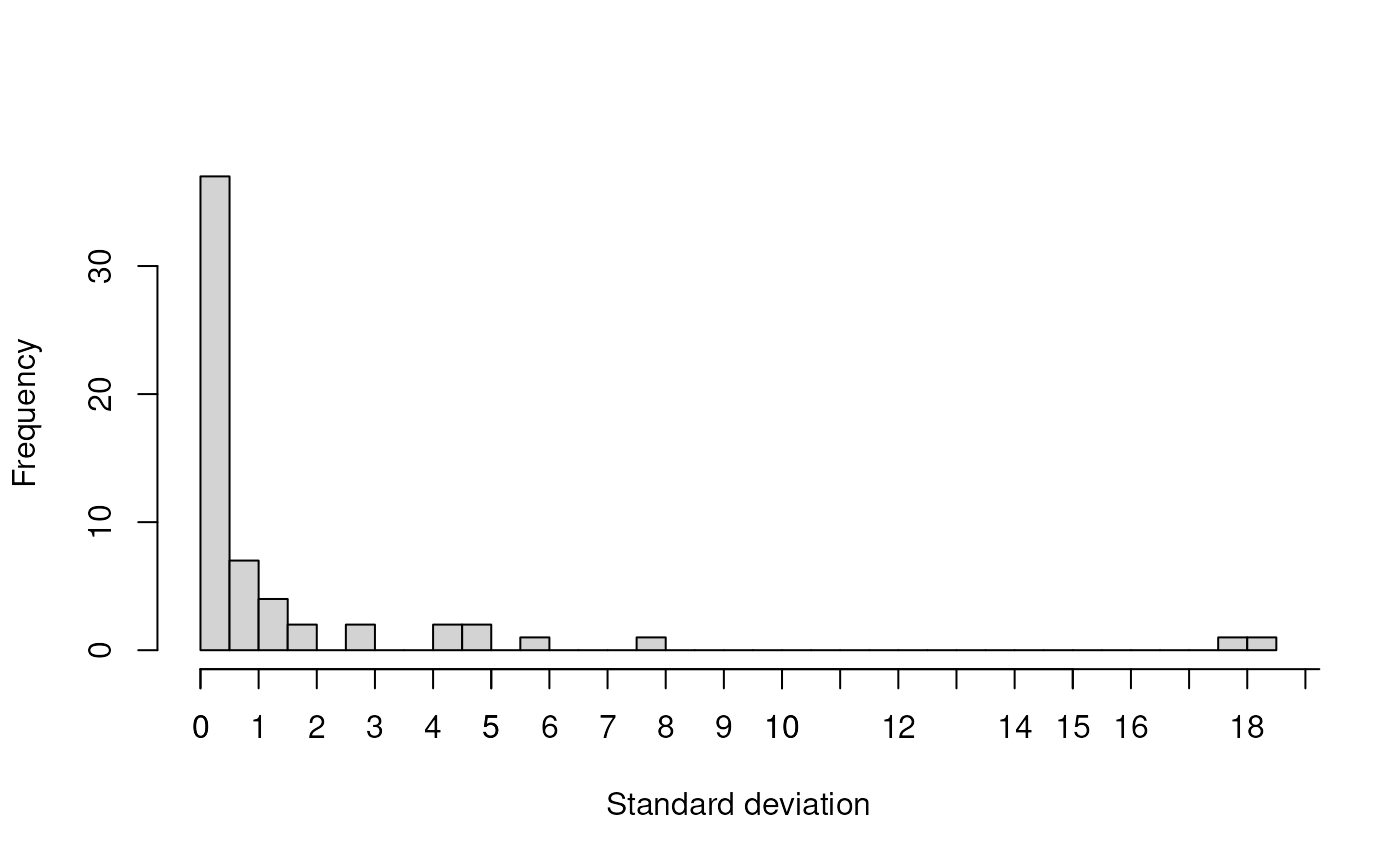
The distribution of standard deviations of fatty acid abundances.
- Percentage of fatty acids with a standard deviation (SD) below 0.5: 61.7%
- Percentage of fatty acids with a standard deviation (SD) below 1: 73.3%
We apply a filtering threshold of 0.5 to exclude fatty acids that do not exhibit sufficient variation in the dataset. Since most standard deviations are below 1, it is a reasonable number if we do not want to exclude too many fatty acids.
mae[[1]] <- mae[[1]][ rowData(mae[[1]])[["sd"]] > 0.5, ]For more detailed analysis, we pick certain fatty acids that have well-established biological relevance. These include:
- Docosahexaenoic acid (DHA)
- Eicosapentaenoic acid (EPA)
- Alpha-linolenic acid
- Arachidonic acid
- Linoleic acid
- Oleic acid
- Palmitic acid
- Stearic acid
relevant_fatty_acids <- c(
    "Docosahexaenoic acid 22:6n-3 (DHA)",
    "Eicosapentaenoic acid 20:5n-3 (EPA)",
    "Alpha-Linolenic acid 18:3n-3",
    "Arachidonic acid 20:4n-6 (ARA)",
    "Linoleic acid 18:2n-6",
    "Oleic acid 18:1n-9",
    "Palmitic acid 16:0",
    "Stearic acid 18:0"
)
altExp(mae[[1]], "relevant") <- mae[[1]][
    rownames(mae[[1]]) %in% relevant_fatty_acids, ]
Transformation
We transform metagenomic counts with relative transformation and centered log-ratio method to tackle the compositional data (see Quinn et al. (2019)).
# Transform microbiome with centered log-ratio method
mae[[2]] <- transformAssay(
    mae[[2]],
    assay.type = "counts",
    method = "relabundance",
    MARGIN = "cols",
    altexp = altExpNames(mae[[2]])
)
mae[[2]] <- transformAssay(
    mae[[2]],
    assay.type = "counts",
    method = "clr",
    pseudocount = TRUE,
    MARGIN = "cols",
    altexp = altExpNames(mae[[2]])
)
#> A pseudocount of 0.5 was applied.
#> A pseudocount of 0.5 was applied.
Fatty acid data is already compositional as it is measured as concentration (mg/g). We apply a log10 transformation to address skewness in the data. Finally, the data is standardized to ensure all features are on a comparable scale.
mae[[1]] <- transformAssay(
    mae[[1]],
    assay.type = "counts",
    method = "log10",
    MARGIN = "cols"
)
mae[[1]] <- transformAssay(
    mae[[1]],
    assay.type = "log10",
    method = "standardize",
    MARGIN = "rows"
)
Analyzing fatty acids: Time and treatment effects
We aim to investigate how fatty acids evolve over time and, more importantly, whether the feed additive impacts these fatty acids. To achieve this, we will fit a simple linear model for each fatty acid, accounting for time and treatment effects in a non-parametric manner. These models resemble the Wilcoxon test but include additional covariates. This approach will allow us to estimate the variability explained by time, treatment, or both factors.
# Get fatty acids that we are going to test
tse <- altExp(mae[[1]], "relevant")

# For each fatty acid, fit linear model
res <- lapply(rownames(tse), function(feat){
    # Get data of single feature
    df <- meltSE(tse[feat, ], add.col = TRUE)
    # Fit model
    res <- lm(rank(counts) ~ study_group + timepoint, data = df)
    # Get only p-values
    res <- summary(res)
    res <- res[[4]][, 4]
    return(res)
})
# Combine results and adjust p-values
res <- do.call(rbind, res) |> as.data.frame()
res <- lapply(res, p.adjust, method = "fdr") |> as.data.frame()
# Add feature names
res[["feature"]] <- rownames(tse)
res |> datatable()
As observed, treatment does not appear to affect fatty acid concentrations significantly. In contrast, time seems to influence nearly all fatty acids; as salmon grow, certain fatty acid concentrations in their muscle tissue increase. This relationship can be further visualized as follows.
p <- plotExpression(
    tse, rownames(tse), assay.type = "counts", x = "timepoint",
    colour_by = "study_group", scales = "free")
p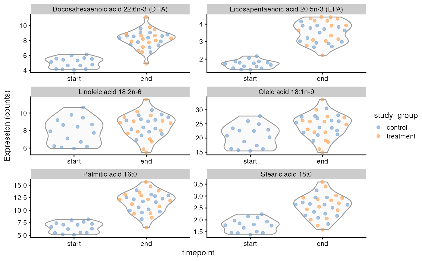
Concentrations of selected fatty acids at the start and end of the trial, with an indication of whether animals received treatment.
Analyzing microbiota: Time and treatment effects
Microbial composition
As a first step in analysing microbiota data, we summarize the microbial composition with relative abundance barplot.
p <- plotAbundance(
    altExp(mae[[2]], "prev_genus"),
    assay.type = "relabundance",
    col.var = c("study_group", "timepoint"),
    facet.cols = TRUE, scales = "free_x"
    ) +
  guides(fill = guide_legend(title = "Genus"))
p
#> Warning: Removed 44 rows containing missing values or values outside the scale range
#> (`geom_bar()`).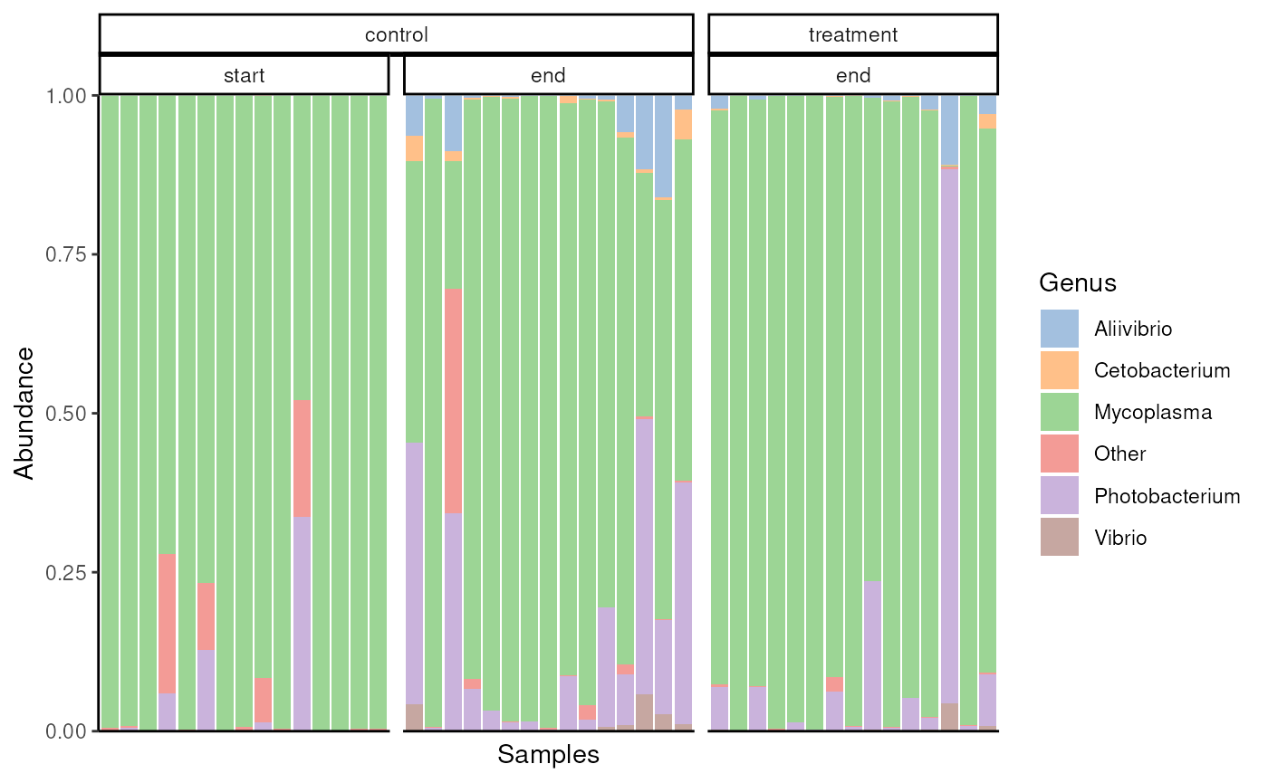
Relative abundance of core microbial genera across samples.
Salmon gut seems to be dominated by either genus Mycoplasma or Photobacterium.
Association of alpha diversity with treatment and salmon age
Now, let’s proceed to calculate the Shannon alpha diversity index.
# Calculate alpha diversity
mae[[2]] <- addAlpha(mae[[2]])
#> Warning: 'faith' index can be calculated only for TreeSE with rowTree(x)
#> populated or with 'tree' provided separately.
With the alpha diversity indices calculated and added to
colData, we can now assess whether time and treatment
influence the microbial diversity in the salmon gut flora.
# Get sample metadata
df <- colData(mae[[2]])
# Fit model to estimate influence of treatment and time to diversity
res <- lm(rank(shannon_diversity) ~ study_group + timepoint, data = df)
res <- summary(res)
res
#>
#> Call:
#> lm(formula = rank(shannon_diversity) ~ study_group + timepoint,
#>     data = df)
#>
#> Residuals:
#>     Min      1Q  Median      3Q     Max
#> -20.933 -10.267  -3.267   9.067  27.200
#>
#> Coefficients:
#>                      Estimate Std. Error t value Pr(>|t|)
#> (Intercept)            16.800      3.138   5.353 3.36e-06 ***
#> study_grouptreatment   -8.333      4.438  -1.878  0.06738 .
#> timepointend           13.467      4.438   3.034  0.00412 **
#> ---
#> Signif. codes:  0 '***' 0.001 '**' 0.01 '*' 0.05 '.' 0.1 ' ' 1
#>
#> Residual standard error: 12.15 on 42 degrees of freedom
#> Multiple R-squared:  0.1826, Adjusted R-squared:  0.1436
#> F-statistic:  4.69 on 2 and 42 DF,  p-value: 0.0145
Based on the results, we conclude that older salmon exhibit distinct microbial diversity compared to younger ones. Additionally, there appears to be a slight — though not statistically significant — effect of treatment on microbial diversity.
p <- plotColData(
    mae[[2]], x = "timepoint", y = "shannon_diversity",
    colour_by = "study_group")
p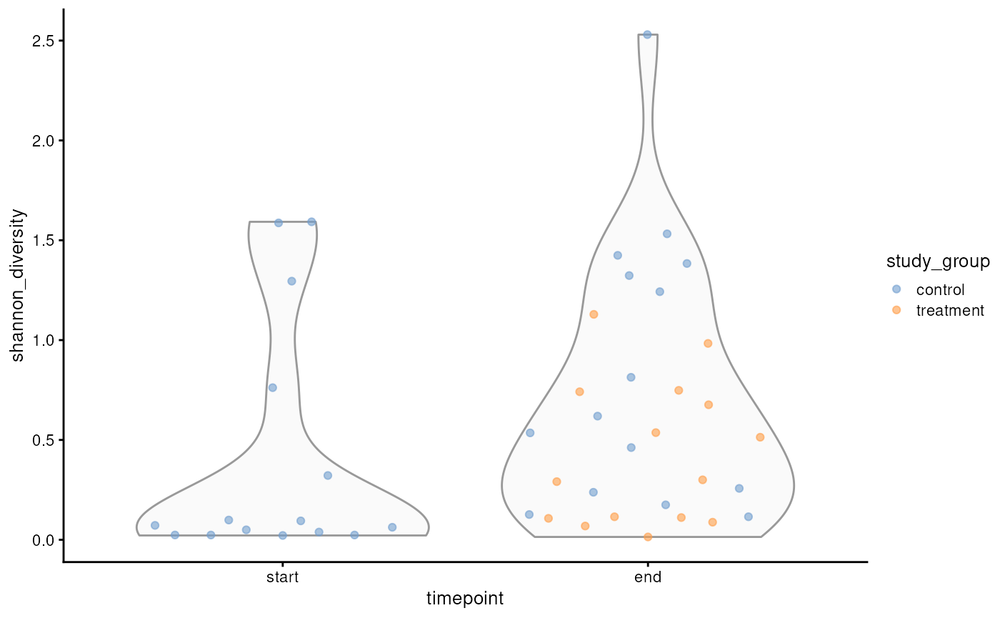
Shannon diversity of microbial communities in salmon at the start and end of the trial, with information on treatment status.
Microbial dissimilarity among samples
Let’s analyze whether we can find similar effect with beta diversity. Here we perform Principal Coordinate Analysis (PCoA) with Bray-Curtis dissimilarity.
# Run PCoA
mae[[2]] <- runMDS(
    mae[[2]],
    FUN = getDissimilarity,
    method = "bray",
    assay.type = "relabundance"
)

# Display dissimilarity on a plot
p <- plotReducedDim(mae[[2]], "MDS", colour_by = "timepoint")
p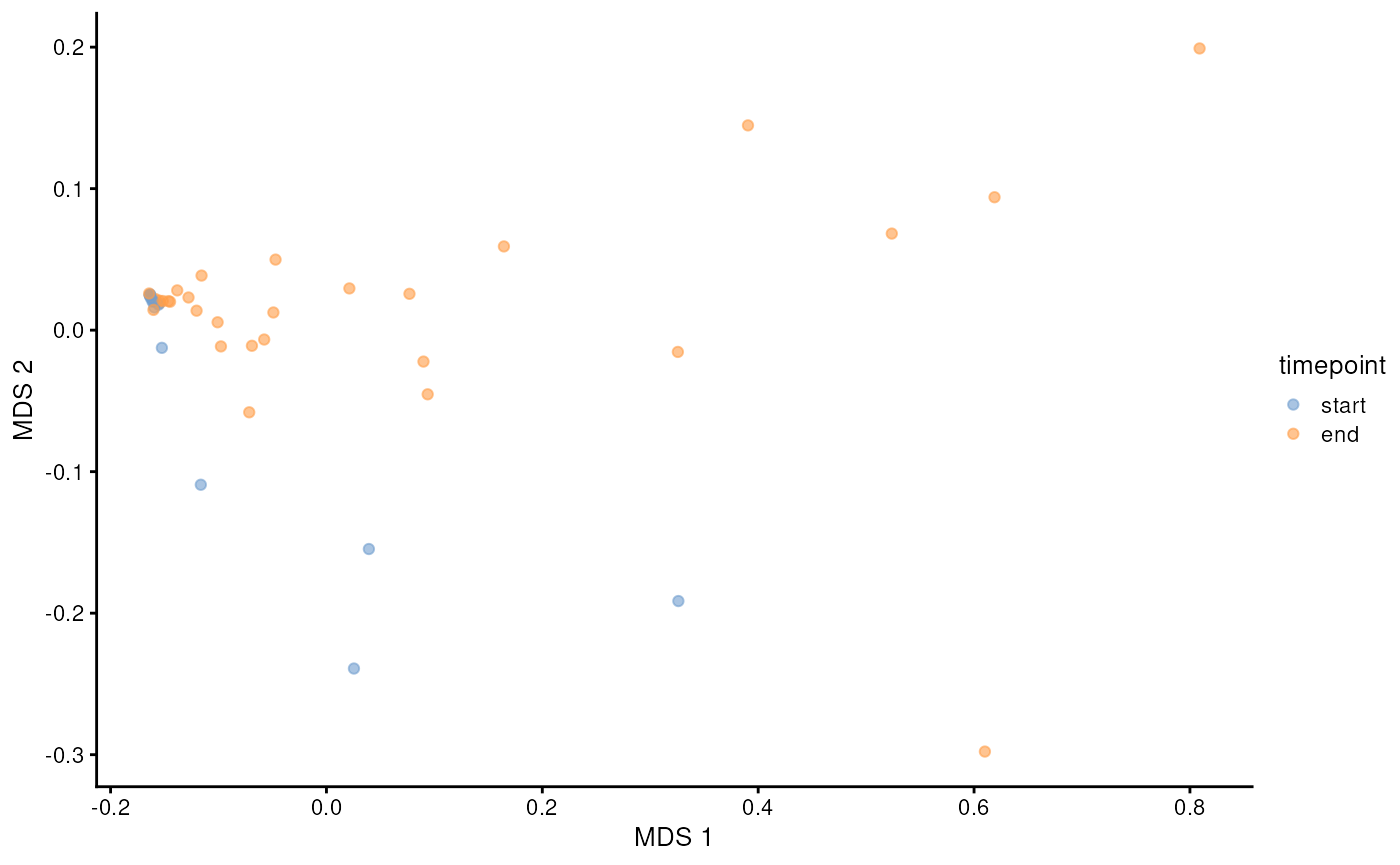
PCoA (Bray-Curtis) of microbial data.
Distinct patterns in the PCoA plot show samples clustering by time points, indicating that microbial profiles vary with salmon age. This reinforces the results observed in alpha diversity, supporting an association between age and shifts in microbial diversity.
Multi-omics integration
Multi-omic factor analysis (MOFA) (see Argelaguet et al. (2020)) allows us to discover latent factors that underlie the biological differences by taking in consideration 2 or more omic assays. To cite the original authors, “MOFA can be viewed as a statistically rigorous generalization of (sparse) principal component analysis (PCA) to multi-omics data”.
By applying MOFA analysis, our goal is to determine whether metagenomics and fatty acids exhibit shared variability, ultimately assessing whether the microbial community is associated with fatty acid composition.
mae_temp <- mae
mae_temp[[2]] <- altExp(mae_temp[[2]], "prev_genus")

# Extract only transformed metagenomic assays for MOFA analysis
assays(mae_temp[[1]]) <- assays(mae_temp[[1]])[
    names(assays(mae_temp[[1]])) %in% c("standardize")
]
assays(mae_temp[[2]]) <- assays(mae_temp[[2]])[
    names(assays(mae_temp[[2]])) %in% c("counts")
]

# Transform MAE object to MOFA model
model <- create_mofa_from_MultiAssayExperiment(mae_temp)

# Set model's options
model_opts <- get_default_model_options(model)
model_opts$num_factors <- 5
model_opts$likelihoods[[2]] <- "poisson"
train_opts <- get_default_training_options(model)
train_opts$maxiter <- 20000

# Change convergence mode to slightly improve accuracy
train_opts$convergence_mode <- "slow"

# Prepare MOFA model
model <- prepare_mofa(
    object = model,
    model_options = model_opts,
    training_options = train_opts
)
#> Warning in prepare_mofa(object = model, model_options = model_opts,
#> training_options = train_opts): Some view(s) have less than 15 features, MOFA
#> will have little power to to learn meaningful factors for these view(s)....
#> Checking data options...
#> No data options specified, using default...
#> Checking training options...
#> Checking model options...

# Train model
model <- run_mofa(model, use_basilisk = TRUE)
#> Warning in run_mofa(model, use_basilisk = TRUE): No output filename provided. Using /tmp/RtmpnACnUH/mofa_20260210-094313.hdf5 to store the trained model.
#> Connecting to the mofapy2 package using basilisk.
#>     Set 'use_basilisk' to FALSE if you prefer to manually set the python binary using 'reticulate'.
#> + /github/home/.pyenv/versions/3.12.12/bin/python3.12 -m venv /github/home/.cache/R/basilisk/1.23.0/MOFA2/1.21.3/mofa_env
#> + /github/home/.cache/R/basilisk/1.23.0/MOFA2/1.21.3/mofa_env/bin/python -m pip install --upgrade pip wheel setuptools
#> + /github/home/.cache/R/basilisk/1.23.0/MOFA2/1.21.3/mofa_env/bin/python -m pip install --upgrade --no-user 'numpy==1.26.4' 'scipy==1.12.0' 'pandas==2.2.1' 'h5py==3.10.0' 'scikit-learn==1.4.0' 'dtw-python==1.3.1' 'mofapy2==0.7.3'
Next, we will plot the variances explained by each factor.
# Plot explained variances
p <- plot_variance_explained(model)
# Get explained variances from model as numeric values
df <- model@cache[[1]][[2]][[1]] |> stack()
df[["percentage"]] <- paste0(round(df[["value"]]), "%")
# Add them to plot
p <- p + geom_shadowtext(aes(label = df[["percentage"]]))
p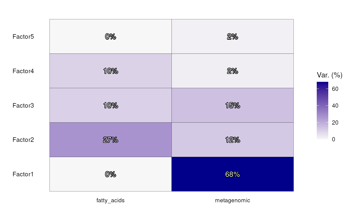
Explained variance by the model for microbial and fatty acid data.
Factor 1 captures only variance within the metagenomics data, while over 2/3 of variance captured by Factor 2 represents variance in fatty acids. Factor 3 captures shared variability between the metagenomic data and fatty acids, reflecting interconnected patterns between the two datasets.
Before exploring the shared variability, we first examine which metagenomic variability is captured by Factor 1. We do not plot fatty acid weights because the captured variability in factor 1 for fatty acids is 0% as seen in the previous plot.
p2 <- plot_top_weights(model, view = 2, factors = 1, nfeatures = 25) +
    labs(title = "Microbiota")

p2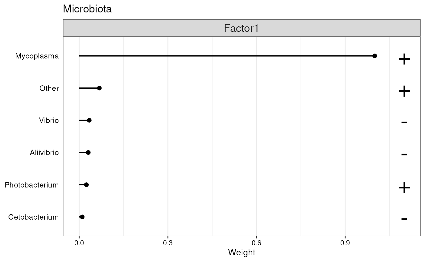
Features with the highest loadings for Factor 1.
From the plot above, we can see that the first factor captures mostly the variability in Mycoplasma.
Let us then focus on loadings of factor 2.
p1 <- plot_top_weights(model, view = 1, factors = 2, nfeatures = 25) +
    labs(title = "Fatty acids")
p2 <- plot_top_weights(model, view = 2, factors = 2, nfeatures = 25) +
    labs(title = "Microbiota")

p1 + p2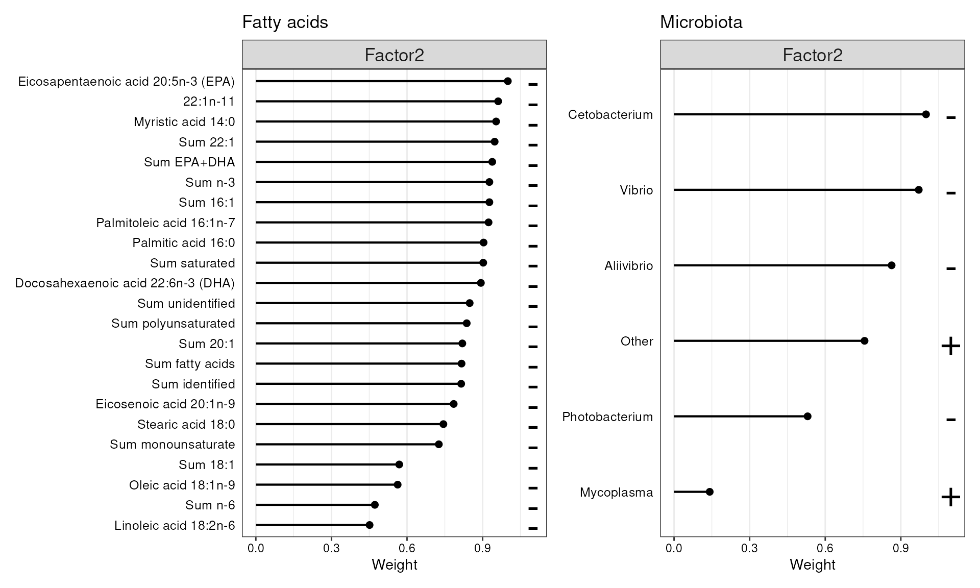
Features with the highest loadings for Factor 2.
In the microbial data, particularly Cetobacterium, Vibrio, and Aliivibrio show a negative association with Factor 2. Additionally, many fatty acids display significant negative weights in this factor, though no single fatty acid can be specifically tied to these taxa. This suggests that as the abundances of these taxa is rise (or decrease), there is a corresponding increase (or decrease) in overall fatty acid levels.
Next, we visualize Factor 3 that captured variance more evenly between microbes and fatty acids.
p1 <- plot_top_weights(model, view = 1, factors = 3, nfeatures = 25) +
    labs(title = "Fatty acids")
p2 <- plot_top_weights(model, view = 2, factors = 3, nfeatures = 25) +
    labs(title = "Microbiota")

p1 + p2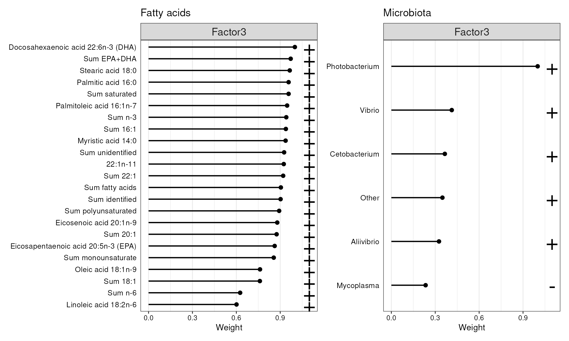
Features with the highest loadings for Factors 3.
From the shared Factor 3, Photobacterium emerge prominently. Similarly to Factor 2, no single fatty acid can be directly associated with any of the microbial species, including Photobacterium.
Worth noting is that, out of these 5 taxa, only Mycoplasma does not appear to share any variability with fatty acids as all its variability was captured by the first factor which did not associate with fatty acids.
Conclusions
The present case study has demonstrated how easy and fast it is to
download large dataset and transform the data into a
MultiAssayExperiment, which in turn gives the researchers
access to an extensive plethora of downstream tools, such
mia and MOFA2 that can be used to pre-process
and visualize the multi-omics data.
Appendix
features <- c(
    "Docosahexaenoic acid 22:6n-3 (DHA)", "Eicosapentaenoic acid 20:5n-3 (EPA)")
tse <- mae[[1]]
tse <- tse[features, ]
rownames(tse) <- c("DHA", "EPA")
p1 <- plotExpression(
    tse, rownames(tse), assay.type = "counts", x = "timepoint",
    colour_by = "study_group", scales = "free", ncol = 1) +
    labs(x = "Time point", y = "Concentration [mg/g]") +
    guides(colour = guide_legend(title = "Study group"))

p2 <- plotAbundance(
    altExp(mae[[2]], "prev_genus"),
    assay.type = "relabundance",
    col.var = c("study_group", "timepoint"),
    facet.cols = TRUE, scales = "free_x"
    ) +
    labs(y = "Relative abundance") +
  guides(fill = guide_legend(title = "Genus"))

p1 + p2  + plot_layout(widths = c(1, 2))
#> Warning: Removed 44 rows containing missing values or values outside the scale range
#> (`geom_bar()`).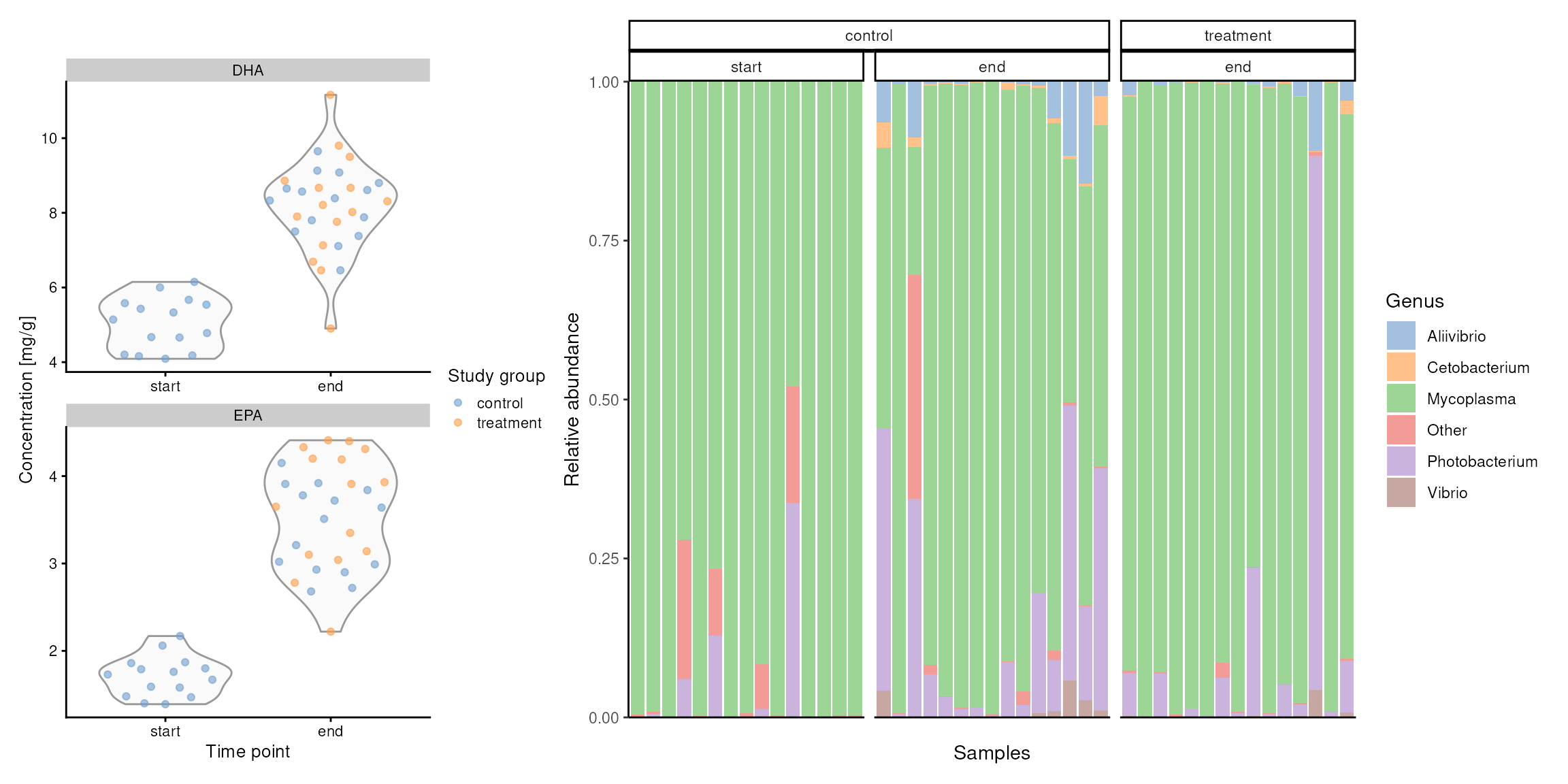
sessionInfo()
#> R Under development (unstable) (2026-02-08 r89382)
#> Platform: x86_64-pc-linux-gnu
#> Running under: Ubuntu 24.04.3 LTS
#>
#> Matrix products: default
#> BLAS:   /usr/lib/x86_64-linux-gnu/openblas-pthread/libblas.so.3
#> LAPACK: /usr/lib/x86_64-linux-gnu/openblas-pthread/libopenblasp-r0.3.26.so;  LAPACK version 3.12.0
#>
#> locale:
#>  [1] LC_CTYPE=en_US.UTF-8       LC_NUMERIC=C
#>  [3] LC_TIME=en_US.UTF-8        LC_COLLATE=en_US.UTF-8
#>  [5] LC_MONETARY=en_US.UTF-8    LC_MESSAGES=en_US.UTF-8
#>  [7] LC_PAPER=en_US.UTF-8       LC_NAME=C
#>  [9] LC_ADDRESS=C               LC_TELEPHONE=C
#> [11] LC_MEASUREMENT=en_US.UTF-8 LC_IDENTIFICATION=C
#>
#> time zone: UTC
#> tzcode source: system (glibc)
#>
#> attached base packages:
#> [1] stats4    stats     graphics  grDevices utils     datasets  methods
#> [8] base
#>
#> other attached packages:
#>  [1] shadowtext_0.1.6                scater_1.39.2
#>  [3] scuttle_1.21.0                  reticulate_1.44.1
#>  [5] patchwork_1.3.2                 MOFA2_1.21.3
#>  [7] miaViz_1.19.1                   ggraph_2.2.2
#>  [9] ggplot2_4.0.2                   mia_1.19.2
#> [11] MGnifyR_1.7.1                   HoloFoodR_1.3.1
#> [13] TreeSummarizedExperiment_2.19.0 Biostrings_2.79.4
#> [15] XVector_0.51.0                  SingleCellExperiment_1.33.0
#> [17] MultiAssayExperiment_1.37.2     SummarizedExperiment_1.41.1
#> [19] Biobase_2.71.0                  GenomicRanges_1.63.1
#> [21] Seqinfo_1.1.0                   IRanges_2.45.0
#> [23] S4Vectors_0.49.0                BiocGenerics_0.57.0
#> [25] generics_0.1.4                  MatrixGenerics_1.23.0
#> [27] matrixStats_1.5.0               ggsignif_0.6.4
#> [29] DT_0.34.0                       dplyr_1.2.0
#> [31] knitr_1.51                      BiocStyle_2.39.0
#>
#> loaded via a namespace (and not attached):
#>   [1] splines_4.6.0               ggplotify_0.1.3
#>   [3] urltools_1.7.3.1            filelock_1.0.3
#>   [5] tibble_3.3.1                triebeard_0.4.1
#>   [7] polyclip_1.10-7             DirichletMultinomial_1.53.0
#>   [9] lifecycle_1.0.5             httr2_1.2.2
#>  [11] lattice_0.22-9              MASS_7.3-65
#>  [13] crosstalk_1.2.2             SnowballC_0.7.1
#>  [15] magrittr_2.0.4              sass_0.4.10
#>  [17] rmarkdown_2.30              jquerylib_0.1.4
#>  [19] yaml_2.3.12                 otel_0.2.0
#>  [21] cowplot_1.2.0               DBI_1.2.3
#>  [23] RColorBrewer_1.1-3          abind_1.4-8
#>  [25] Rtsne_0.17                  purrr_1.2.1
#>  [27] yulab.utils_0.2.4           tweenr_2.0.3
#>  [29] rappdirs_0.3.4              gdtools_0.5.0
#>  [31] ggrepel_0.9.6               irlba_2.3.7
#>  [33] tokenizers_0.3.0            tidytree_0.4.7
#>  [35] pheatmap_1.0.13             vegan_2.7-2
#>  [37] pkgdown_2.2.0               permute_0.9-10
#>  [39] DelayedMatrixStats_1.33.0   codetools_0.2-20
#>  [41] DelayedArray_0.37.0         ggforce_0.5.0
#>  [43] tidyselect_1.2.1            aplot_0.2.9
#>  [45] farver_2.1.2                ScaledMatrix_1.19.0
#>  [47] viridis_0.6.5               jsonlite_2.0.0
#>  [49] BiocNeighbors_2.5.3         decontam_1.31.0
#>  [51] tidygraph_1.3.1             systemfonts_1.3.1
#>  [53] tools_4.6.0                 ggnewscale_0.5.2
#>  [55] treeio_1.35.0               ragg_1.5.0
#>  [57] Rcpp_1.1.1                  glue_1.8.0
#>  [59] BiocBaseUtils_1.13.0        gridExtra_2.3
#>  [61] SparseArray_1.11.10         xfun_0.56
#>  [63] mgcv_1.9-4                  HDF5Array_1.39.0
#>  [65] withr_3.0.2                 BiocManager_1.30.27
#>  [67] fastmap_1.2.0               ggh4x_0.3.1
#>  [69] basilisk_1.23.0             rhdf5filters_1.23.3
#>  [71] bluster_1.21.0              digest_0.6.39
#>  [73] rsvd_1.0.5                  R6_2.6.1
#>  [75] gridGraphics_0.5-1          textshaping_1.0.4
#>  [77] h5mread_1.3.1               ecodive_2.2.2
#>  [79] UpSetR_1.4.0                tidyr_1.3.2
#>  [81] fontLiberation_0.1.0        DECIPHER_3.7.0
#>  [83] graphlayouts_1.2.2          httr_1.4.7
#>  [85] htmlwidgets_1.6.4           S4Arrays_1.11.1
#>  [87] uwot_0.2.4                  pkgconfig_2.0.3
#>  [89] gtable_0.3.6                S7_0.2.1
#>  [91] janeaustenr_1.0.0           htmltools_0.5.9
#>  [93] fontBitstreamVera_0.1.1     bookdown_0.46
#>  [95] scales_1.4.0                png_0.1-8
#>  [97] corrplot_0.95               ggfun_0.2.0
#>  [99] reshape2_1.4.5              nlme_3.1-168
#> [101] cachem_1.1.0                rhdf5_2.55.13
#> [103] stringr_1.6.0               parallel_4.6.0
#> [105] vipor_0.4.7                 desc_1.4.3
#> [107] pillar_1.11.1               grid_4.6.0
#> [109] vctrs_0.7.1                 BiocSingular_1.27.1
#> [111] beachmat_2.27.2             cluster_2.1.8.2
#> [113] beeswarm_0.4.0              evaluate_1.0.5
#> [115] cli_3.6.5                   compiler_4.6.0
#> [117] rlang_1.1.7                 crayon_1.5.3
#> [119] tidytext_0.4.3              labeling_0.4.3
#> [121] forcats_1.0.1               plyr_1.8.9
#> [123] fs_1.6.6                    ggbeeswarm_0.7.3
#> [125] ggiraph_0.9.4               stringi_1.8.7
#> [127] viridisLite_0.4.3           BiocParallel_1.45.0
#> [129] lazyeval_0.2.2              fontquiver_0.2.1
#> [131] Matrix_1.7-4                dir.expiry_1.19.0
#> [133] sparseMatrixStats_1.23.0    Rhdf5lib_1.33.0
#> [135] igraph_2.2.1                memoise_2.0.1
#> [137] bslib_0.10.0                ggtree_4.1.1
#> [139] ape_5.8-1